


Up: Brownian Motion and Focker-Planck
Previous: Langevin Equation
Subsections
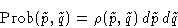
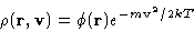
In equilibrium thermodynamics we introduced distribution
function  : the probability to have
momenta around
: the probability to have
momenta around  and coordinates around
  is
is
- We will study one Brownian particle--one coordinate
 and one velocity
- We want a time-dependent solution--we must introduce t
We introduce a time-dependent distribution function
 --the probability to be in certain place with
certain velocity at certain time!
--the probability to be in certain place with
certain velocity at certain time!
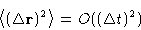
If the Brownian motion is the slowest mode in the system, there exists
such time  that:
that:
- 1.
- is large enough, so there are many molecular
collisions during this time
- 2.
- is small enough, so and do not change
``much''
We know the state of our particle at time t: and . What
is its state at the time  ?
?
- Assumption:
- The state of the system at the moment depends only on the state at the moment t. The system has
short memory.
- Definition:
- A system satisfying this assumption is called
Markov system. We assume Brownian motion to be Markovian.
We introduce 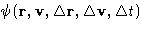 --the probability
to go from state 1 to state 2:
--the probability
to go from state 1 to state 2:
![\begin{displaymath}
\mathbf{r},\mathbf{v}\xrightarrow[\Delta
t]{\psi(\mathbf{r}...
...lta t)} \mathbf{r}+\Delta\mathbf{r},\mathbf{v}+\Delta\mathbf{v}\end{displaymath}](img37.gif)
or, introducing the variable 
![\begin{displaymath}
u\xrightarrow[\Delta
t]{\psi(u,\Delta u,\Delta t)} u+\Delta u\end{displaymath}](img39.gif)
The function  is called transfer function. The evolution
of Markov system depends only on transfer function and initial state.
is called transfer function. The evolution
of Markov system depends only on transfer function and initial state.
Whatever is the state you started from, you will finish at some state
with probability 1![[*]](/icons/foot_motif.gif) :
:
| 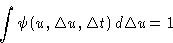 |
(8) |
What is the probability to find particle at the point u at the
time ? If it was at the point  at time t, the
probability is
at time t, the
probability is 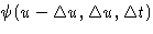 . The probability to
be at was
. The probability to
be at was  . We obtain:
| 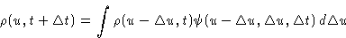 |
(9) |
This is called Chapman-Kolmogorov (or master) equation.
Now we will use the fact that is small. In the left hand
side of (9) we have:
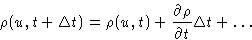
In the right hand side (do not forget that u is a vector!):
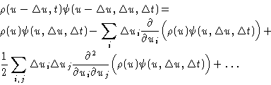
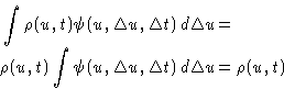
Integration:
- 1.
- First term gives
- 2.
- Second term gives:
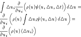
- 3.
- Third term gives:
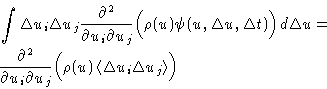
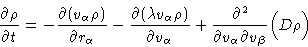
We obtained:
| 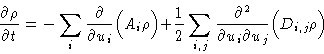 |
(10) |
with drift coefficients

and diffusion coefficients
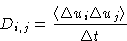
This is called Focker-Planck equation. It describes
diffusion in phase space.
The evolution is described by the moments  . In the Focker-Planck equation we use only the first and
second moments. In principle, we can construct an approximation
based on higher moments (Kramers, 1940).
. In the Focker-Planck equation we use only the first and
second moments. In principle, we can construct an approximation
based on higher moments (Kramers, 1940).
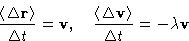
For Brownian motion we have:
- 1.
- Linear terms are
- 2.
- Cross terms are zero:

- 3.
- Quadratic in term is:
- 4.
- Quadratic in term is
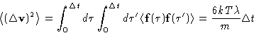
Result (summation over  &
&  is implied):
with

If viscosity is large, we can assume that quickly relaxes to
equilibrium value:
Integrating Focker-Planck equation, we can obtain diffusion equation

Up: Brownian Motion and Focker-Planck
Previous: Langevin Equation
© 1997
Boris Veytsman
and Michael Kotelyanskii
Sun Nov 2 18:50:28 EST 1997