Next: NPT Ensemble Up: Calculation of Thermodynamic Properties. Previous: Calculation of Thermodynamic Properties.

Thermodynamic Properties in NVT Ensemble

Pressure.

As we pointed out in the beginning of this chapter, the main purpose of the computer simulations is to calculate thermodynamic properties. They are calculated as averages of the corresponding functions that depend on the particle coordinates. The averaging is done over the configurations, produced during the MC run.

For many quantities, like magnetization or energy, the calculations are obvious. Pressure is a little more tricky, and now we are going to derive the expression for it.

As we remember from the thermodynamics:

$\begin{displaymath} p=kT\left( \frac{\partial \log Z}{\partial V}\right)_{N,T}\end{displaymath}$

where

$\begin{displaymath} Z= \int_0^V d\mathbf{r}_1 \dots \int_0^V d\mathbf{r}_N\, \exp\bigl(-\beta U(\mathbf{r}_1\dots\mathbf{r}_N)\bigr) \end{displaymath}$

For simplicity, we assume, that the simulation cell has cubic shape, and make the coordinate change

$\begin{displaymath} x'=\chi x, \quad y'= \chi y, \quad z' = \chi z, \quad \chi=V^{-1/3}\end{displaymath}$

Then the coordinate $\alpha$ of the particle i is ${\mathbf{r}'}_i^{\alpha} = \chi \mathbf{r}_i^{\alpha}$ , and

$\begin{displaymath} \begin{aligned} \left( \frac{\partial Z}{\partial V} \righ... ...ft(-\beta U\right) \frac{\partial U}{\partial V} \end{aligned}\end{displaymath}$

(1)

with

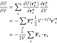
$\begin{displaymath} \begin{aligned} \frac{\partial U}{\partial V}&=\sum_{i} \fra... ...1}{3V}\sum_{i}\mathbf{F}_{i}\cdot\mathbf{r}_{i} \end{aligned}\end{displaymath}$

(2)

Now after going back to the initial coordinates and substituting $\partial\log Z_N/\partial V=Z_N^{-1}\partial Z_N/\partial V$ , we see, that the first term is just density, and the second is an ensemble average of the sum of the force times coordinate.

$\begin{displaymath} pV = Nk_BT - \langle \frac{1}{3}\sum_i\mathbf{F}_{i}\cdot\mathbf{r}_{i} \rangle\end{displaymath}$

The second term on the right hand side is called virial, and this equation is often called the virial equation. If the interaction potential is pairwise, it can be rearranged as follows:

$\begin{displaymath} \begin{gathered} U(\mathbf{r}_{i}^{\alpha})= \sum_{i\neq j} ... ...sum_{j\neq i} \mathbf{r}_{i}\cdot \mathbf{F}_{ij}\end{gathered}\end{displaymath}$

$\mathbf{F}_{ij}$ is the force, acting on the atom i from the atom j. $\mathbf{F}_{ij} = - \mathbf{F}_{ji}$ (Why?).

$\begin{displaymath} \begin{aligned} \sum_i\mathbf{F}_{i}\cdot\mathbf{r}_{i} &= \... ...m_i \sum_{j\gt i} r_{ij}\frac{dv(r_{ij})}{dr_{ij}}\end{aligned}\end{displaymath}$ (3)

Finally, we obtain

$\begin{displaymath} pV=Nk_BT+\frac{1}{3}\langle \sum_i \sum_{j\gt i} r_{ij}\frac{dv(r_{ij})}{dr_{ij}} \rangle\end{displaymath}$ (4)

Equation 4 should look familiar. Before, when we discussed the theory of liquids , we derived the same expression for pressure but in terms of the pairwise interaction potential and g(r). Here we derived more general expression, applicable even in the case when the interactions are not necessarily pairwise. It also does not require calculations of g(r), that can be very involved.

Chemical potential

If we have a system of N particles at temperature T, and volume V, the chemical potential $\mu$ at large enough N can be written as:

$\begin{displaymath} \exp(-\beta \mu) = Q_{N+1}/Q_N = Q_N/Q_{N-1}\end{displaymath}$

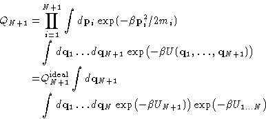
where Q_N is partition function for the system of N particles in the volume N. The $\{N+1\}$ -particle partition function is:

$\begin{displaymath} \begin{aligned} Q_{N+1} =& \prod_{i=1}^{N+1} \int d\mathbf{... ...{N+1})\bigr) \exp\bigl(-\beta U_{1\dots N}\bigr)\end{aligned}\end{displaymath}$

(5)

Here we split the total system energy into the interaction U_N+1 of the N+1-st particle with the other N particles, and the energy $U_{1\dots N}$ of the N-particle system. The integral in the last equation can be rewritten as the ensemble average of $\exp(-\beta U_{N+1})$ over the ensemble of systems with N particles:

$\begin{displaymath} \exp(-\beta \mu) = Q_{\text{ideal}} \langle \exp(-\beta U_{N+1})\rangle_N \end{displaymath}$

This is the basis for the so-called

Widom test-particle method.

Perform NVT MC simulation for the system of N particles
Calculate the average of the $\exp(-\beta U_{N+1})$ , by inserting the ``ghost'' particle at random positions inside the box, and calculating its interaction energy with the rest of the system, as if it were real.

This technique works fine at moderate densities around the critical point, but turns out to have problems at high densities around liquid-solid coexistence, because the probability to insert the ``ghost'' at the place where the $\exp(-\beta U_{N+1})\ne0$ is very small.

Pair distribution function g(r)

The importance of the pair distribution function g(r) was discussed in the chapter on the liquid-state theory . Its calculation in the MC simulations is really straightforward. All we have to do is just to count the number of particles at the distances between r and r+dr from the chosen particle. In the homogeneous systems it is also averaged over all particles. It is calculated as a histogram with the bin width dr, and then is normalized by the area of the spherical layer.

Code example: (to be added to the MC code). Notice, that it is 2D! Code.

Long-Range Corrections

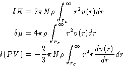
In the previous lecture we mentioned, that it is very convenient to cut the interaction potential after certain cut-off distance r_c. The thermodynamics properties has to be corrected for this approximation. The expressions are listed below:

$\begin{displaymath} \begin{aligned} \delta E & = 2\pi N \rho \int_{r_c}^{\infty}... ...rho \int_{r_c}^{\infty} r^2 r \frac{dv(r)}{dr} dr \end{aligned}\end{displaymath}$

(6)

Next: NPT Ensemble Up: Calculation of Thermodynamic Properties. Previous: Calculation of Thermodynamic Properties.