NPH and NPT MD

We have already seen in Monte Carlo , that isobaric simulations should involve volume changes. So constant pressure MD naturally involves the volume changes and its implementation requires the equation of motion to describe its evolution. The technique described below was proposed by Andersen in 1980, and involves coordinates scaling, similar to NPT Monte Carlo, described previously.

First we introduce the constant pressure analog of the microcanonical ensemble--iso-enthalpic ensemble. We already know, how to make it work at a constant temperature. Now we will show how to make P constant.

Constant pressure is realized by the virtual ``piston'' of mass M (which actually has units of $\text{(mass)}\text{(length)}^{-4}$), which is under constant force, that corresponds to the applied pressure P₀. Piston motion changes the volume of the system. Additional kinetic $M \dot{V}^2/2$ and potential P₀V energy terms, coupled to the particles' momenta, are added to the Hamiltonian (Hoover, 1985). The potential and kinetic energies of the particles are written in terms of scaled variables $\mathbf{s}_i$ and $\dot{\mathbf{s}_i}$

$$\mathbf{r}_i = V^{1/3} \mathbf{s}_i, \mathbf{v}_i = V^{1/3} \dot{\mathbf{s}_i}$$ (10)

Using Hamilton equations (4) for the total Hamiltonian, we obtain:

$$\begin{aligned} \ddot{\mathbf{s}_i}=&\mathbf{F}_i/(m_iV^{1/3... ...)\dot{\mathbf{s}_i}\dot{V}/V\ \ddot{V}=&(P-P_0)/M\end{aligned}$$ (11)

P is the instantaneous value of pressure, calculated via the usual virial expression. The total Hamiltonian is conserved, and is actually equal to the system enthalpy plus kinetic energy of the ``piston'', associated with the volume fluctuations. The mass of the virtual piston M determines the relaxation rate of the volume.

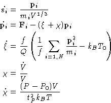
Coupling this method to the Hoover thermostat by introducing another variable $\eta$ (and $\xi=\dot{\eta}$), we can make the whole thing reproduce the NPT ensemble. This can be again shown using Liouville equation for the probability density distribution. NPT-MD equations are:

$$\begin{aligned} \dot{\mathbf{s}_i} &= \frac{\mathbf{p}_i}{m_... ...V}}{V}\ \dot{\chi} &=\frac{(P-P_0)V}{t_P^2 k_B T}\end{aligned}$$ (12)

Here we introduce the parameter t_P instead of ``piston'' mass M. It describes characteristic time of volume relaxation.

Again a non-rigorous, but practical scheme, similar to the van Gunstern-Berendsen thermostat exists. It is called Berendsen barostat. It rescales the particle coordinates at every step by the factor

$$\chi=1-\frac{\delta t}{t_P}(P_0-P)$$ (13)

It is much easier to program and does not has a strong effect on the trajectories, if used carefully. This makes it very practical. This method and van Gunstern-Berendsen thermostat are widely used in simulations, because both methods involve velocities in the right hand sides of the equations of motion, which makes Verlet algorithm still usable, but not as exact as in the microcanonical ensemble. The rigorous methods are often used with more expensive predictor-corrector integrators.