Subsections

• Stochastic Method
• Velocity rescaling
• Coupling to the External Degree of Freedom. Hoover Thermostat

Constant Temperature MD

Stochastic Method

How can we make a transition from the constant energy to the constant temperature? By coupling to the environment, or to the thermal bath.

Coupling to the environment is simulated by random ``collisions'' with imaginary heat bath particles. These collisions lead to instantaneous momentum changes. The particle momenta are reset to new values, taken from the Maxwell distribution. This way the average kinetic energy is always right.

The natural variation on this theme is resetting velocities of all particles at the same time after certain interval. Then the dynamics during this interval is truly microcanonical, and time correlation functions can be calculated inside this interval.

After the new velocities are assigned, the new configuration is accepted or rejected based on Metropolis-like criteria for Monte Carlo simulations. This technique was first suggested by Heyes in 1980, and then reinvented by D. Heermann et. al. in 1990 as Hybrid Monte Carlo. D. Heermann et. al. also showed, that this acceptance criterium is needed to account for the numerical integration errors. Otherwise this technique reproduces canonical ensemble only approximately.

Velocity rescaling

An alternative way to simulate constant temperature is to rescale all the velocities to keep kinetic energy constant. It is a very crude approach used in the early days. If done on every step, it alters the system dynamics, which does not even correspond to the canonical ensemble (Why?). If done at certain intervals, it adds some periodic perturbation to the system, which is in general undesirable, but sometimes can serve as a tool to study system dynamics. Was used for simulations of glasses by Rahman et. al. in early 1980's. It is also often used to equilibrate the system during the the first few hundred MD steps before the production run starts and data are collected.

A more gentle and more practical way, known as van Gunstern-Berendsen thermostat is to use a factor, that depends on the deviation of the instantaneous kinetic energy K from the average value K₀, corresponding to desired temperature T₀. At each time step velocities are scaled by the factor $\chi$:

$$\chi^2 = 1 + \frac{\delta t}{\tau} \left(\frac{K_0}{K}-1 \right)$$ (7)

$\delta t$ is the MD time step, and $\tau$ is a parameter, that defines, how strong is the thermostat influence.

Although this method does not reproduce canonical ensemble, it is widely used, and usually gives the same results as the rigorous method discussed below, although the caution must be taken using it. It reproduces the correct average energy, but the distribution is wrong. Therefore, averages are usually correct, but fluctuations are not.

Coupling to the External Degree of Freedom. Hoover Thermostat

This method does reproduce canonical ensemble, even though it also involves velocity rescaling.

The idea is to introduce an additional degree of freedom $\eta$,describing the external bath and corresponding velocity $\xi=\dot{\eta}$. Additional kinetic $\frac{Q \xi^2}{2}$, and potential $\eta \sum_{i=1,N}\frac{\mathbf{p}_i^2}{2m_i}-\frac{3}{2}k_B T_0$energy terms, coupled to the particles momenta, are added to the Hamiltonian (Hoover, 1985). Using Hamilton equations (4) we obtain equations of motion:

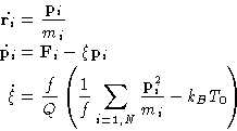$$\begin{aligned} \dot{\mathbf{r}_i} &= \frac{\mathbf{p}_i}{m_... ..._{i=1,N}\frac{\mathbf{p}_i^2}{m_i}-k_B T_0 \right)\end{aligned}$$ (8)

f here is the total number of degrees of freedom in the system. The whole system, that contains all ``real'' degrees of freedom plus $\eta$ and $\xi$ is conservative, and obeys Liouville equation. It can be shown by direct substitution (see homework problem), that the canonic distribution

$$\rho \sim \exp\left[-\beta \left(\sum_{i=1,N}\frac{\mathbf{p}_i^2}{2m_i}+U({\mathbf{q}_1\dots\mathbf{q}_N})\right)\right]$$ (9)

is its stationary, time independent solution. Therefore, configurations sampled by this algorithm represent canonical ensemble.

There is an alternative, but very similar method, called Nose thermostat, which also uses an additional variable for the momenta rescaling. It was introduced earlier (Nose, 1984). It works in the scaled coordinates, and reproduces canonical distribution for positions and scaled momenta.