Subsections

• MC for Ising model
• Simulating Infinite System. Periodic Boundaries

Ising Model

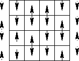
This is a pet model to study phase transitions. It has been introduced before when we discussed phase transitions. It is the lattice of spins, interacting via the nearest neighbor interaction -Js₁ s₂. We consider here cubic lattice and the simplest model with $s_i=\pm1$.This model is fairly simple to simulate, and at the same time provides good illustration of how does the MC method work for multi-particle systems.

• Phase space is discrete, $\{s_i\}$ - set of the spin-states for the lattice sites.
• The total energy is: $U(\{s_i\}) = J \sum_i s_i \sum_{\text{neighbor $j$}} s_j$

Average magnetization $m= \sum_i s_i/N$ is zero at T>T_c, and has some non-zero value m(T) at T<T_c, where T_c is a Curie temperature, or an upper critical point, if we map the fluid mixture on the Ising model.

Two following figures show the results for a 3D Ising model from the MC simulations.

$$\mbox{\rotatebox{-90}{\includegraphics[width=4in]{ising.m.xmgr.plot.eps}}}$$

$$\mbox{\rotatebox{-90}{\includegraphics[width=4in]{ising.m2.xmgr.plot.eps}}}$$

Notice, that critical temperature is determined by the location of the susceptibility maximum. When determined this way it also reflects the system size effects on the criticality.

A method to correct for the system size effects is described in works by K. Binder and coworkers. Very good description can be found in the book by K. Binder and D. W. Heermann ``Monte Carlo Simulations in Statistical Physics'' It involves calculations of the high-order moments of the order parameter distributions, that require very long simulations and use tricks to speed up the calculations. This is beyond the scope of this course.

MC for Ising model

1.

Choose the initial configuration of the system, calculate energy

2.

Loop through the lattice:

• Pick the lattice site i to swap, calculate the energy change if swapped (s_i=-s_i): $\Delta U = -2J \sum_{\text{neighbor $j$}} s_j$.
• Decide whether to accept the move, based on the Metropolis criterium:
• if $\delta U \gt 0$, calculate $w=\exp(-\beta \delta U)$
• draw a random number r from 0 to 1.
• if w<r or $\delta U \leq 0$, swap s_i=-s_i, update the total magnetization and the energy,
• go back to the beginning of the lattice loop

3.

update current values of the running averages.

4.

go back to step 2

Fortran code Example 4 :

Here is an example of the Fortran code for the 2D Ising model on the $N\times N$ lattice. Notice that this model simulates a system of finite size. Code.

Simulating Infinite System. Periodic Boundaries

The previous example (3) deals with the finite system with boundaries. As it will be seen from the homework this has a huge size effect, due to the fact that sites on the border have no neighbors. This is exactly surface tension contribution to the free energy. How can we go around this, if we want to simulate bulk system where the surface effects are negligible? The size of the system that we can simulate is restricted by the computer resources, so we have to somehow simulate the effect of the surrounding material on the simulated region.

Stochastic Boundaries

We can surround the simulated region by the layers of spins, that are taken randomly from inside the system, e.g. if we have 2D lattice of N_x N_y spins, we make up two additional columns at x=0,N_x +1, and two more rows at y=0,N_y+1, and set the spin states in this columns (rows), from the configuration of the randomly chosen inner column (row), at one of the previous system configurations, that is also chosen at random. of our system

Periodic Boundaries

This is the most popular way, used in almost all the simulations in the bulk systems, not only for lattice simulations. Here we again add two additional columns (rows), but the extra column at x=0 has all its spins at the same states as the column at x=N_x, x=N_x+1 is the same as x=1 (Fig. 1). Similar for the border in the y-direction (see the first Quiz problem).

  

Figure 1: Periodic boundaries for the 2D Ising $4\times4$ lattice.